It is very common in real-life systems to see signals being combined in a process known as additive mixing, sometimes referred to as simply mixing, summation, addition or interference. Examples include your computer playing a notification sound on top of your music or reducing the number of channels from an audio stream before playback (downmixing); however the most complex — and most intriguing — examples come from the acoustic realm, in which sound from multiple sources combine at a given point in space. [note] In real-world home audio systems this happens literally all the time. If you’re not convinced, consider that sound bounces off walls, and the interference that this produces has huge implications for acoustics. But that’s a story for another post. [end note]
For the sake of this discussion, we’ll assume that the system that is combining these signals is, for all intents and purposes, linear. In the digital and analog realms this a safe assumption to make as long as non-linear distortion is kept in check. In particular the peak amplitude of the resulting signal needs to be low enough to avoid clipping. [note] In fact, you might be compelled to use the calculations described below precisely to ensure that you won’t drive your system into clipping; indeed this is a common concern when mixing signals digitally or electronically. [end note] To a much lesser extent, this also applies to the acoustic realm: air can be assumed to be linear insofar as we’re not dealing with extreme eardrum-busting pressures. [note] The textbook case where that assumption breaks is when large amounts of sound energy are forced down a narrow tube. One example is the throat (i.e. the loudspeaker-facing part) of the horn in a horn loudspeaker, which is subject to enormous dynamic pressures from the compression driver. (See Kleiner, Eargle, Thuras.) [end note]
What’s nice about linear systems is that they follow the superposition principle: summing two signals can be done, quite literally, by taking the values of both waveforms at a given point in time and adding one to the other. It’s as simple as that (just don’t forget about the sign). That being said, it would be nice to have a general idea of what to expect when summing waves of specific shapes. This is especially important in cases where the two signals being mixed might be related to each other, as is often the case. I’ll start with very simple scenarios and make my way to the less trivial cases.
Same frequency, same phase
Let’s say we want to sum two pure sine waves of identical frequency and phase. [note] It is important that the frequencies match exactly, otherwise you will end up with a surprising (and counter-intuitive) pattern called a beat. Fortunately this is rarely a problem in practice because in a typical home audio system all signals use a consistent timing reference (often originating from a single digital clock signal), which means their frequencies are always in precise lockstep. [end note]
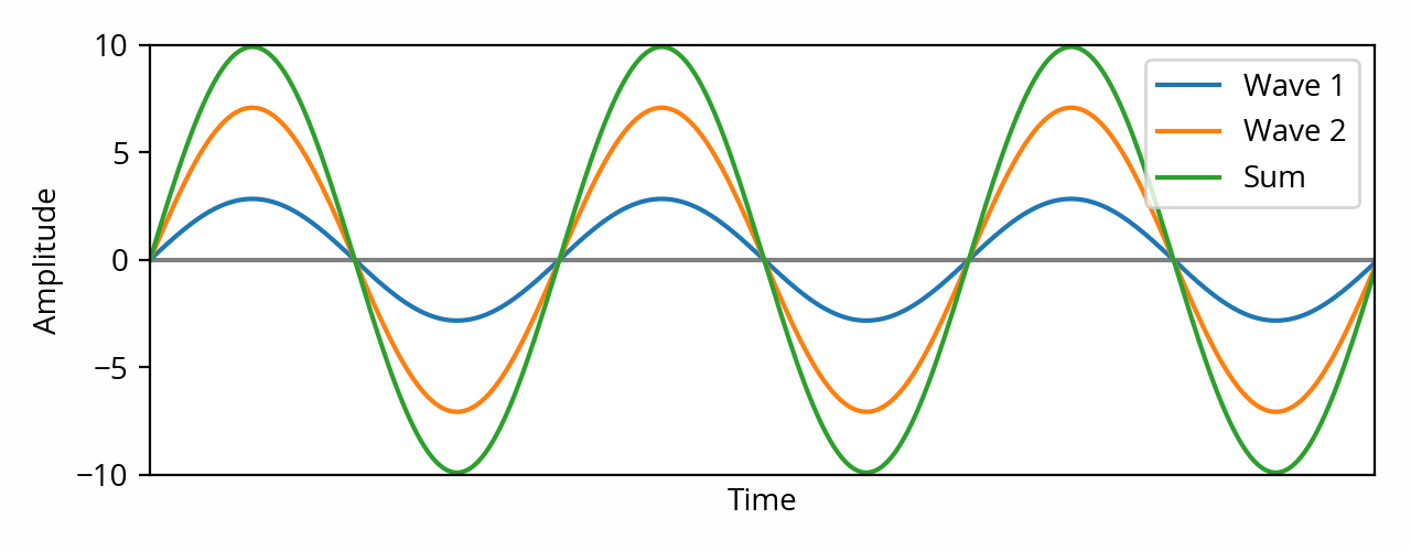
The above plot illustrates the fact that when two sines of identical frequency are mixed together, the result is always a sine of that same frequency. [ref] This follows from mathematical properties of sines. [end ref] Furthermore, in this particular example, the peaks of the two sine waves are aligned because they have the same phase. Since they’re aligned, it follows naturally that the peak amplitude of the resulting signal is simply the sum of the peak amplitudes of the two original signals.
We’ve seen previously that the RMS amplitude of a sine wave is simply its peak amplitude divided by a constant, so we can in turn deduce that the RMS amplitude of the resulting signal is the sum of the RMS amplitudes of the original signals. The resulting amplitude is higher than the amplitudes we started with, which is why this is called constructive interference. [note] The general concepts of constructive and destructive interference are not limited to sine waves. They can be used to describe the interaction between any waveforms as long as they are coherent. Two sine waves of identical frequency are always coherent. Note that there seems to be a lot of confusion around the terms “coherent” and “in phase”. According to the Wikipedia definition two coherent waveforms do not necessarily have the same phase, yet the term “coherent sum” is often thrown around to specifically describe perfect constructive interference. [end note]
The sum of two sine waves that have identical frequency and phase is itself a sine wave of that same frequency and phase. The resulting amplitude (peak or RMS) is simply the sum of the amplitudes.
Same frequency, opposite phase
Now let’s take the same scenario as above, but this time one of the two waves is 180° out of phase, i.e. it is inverted.
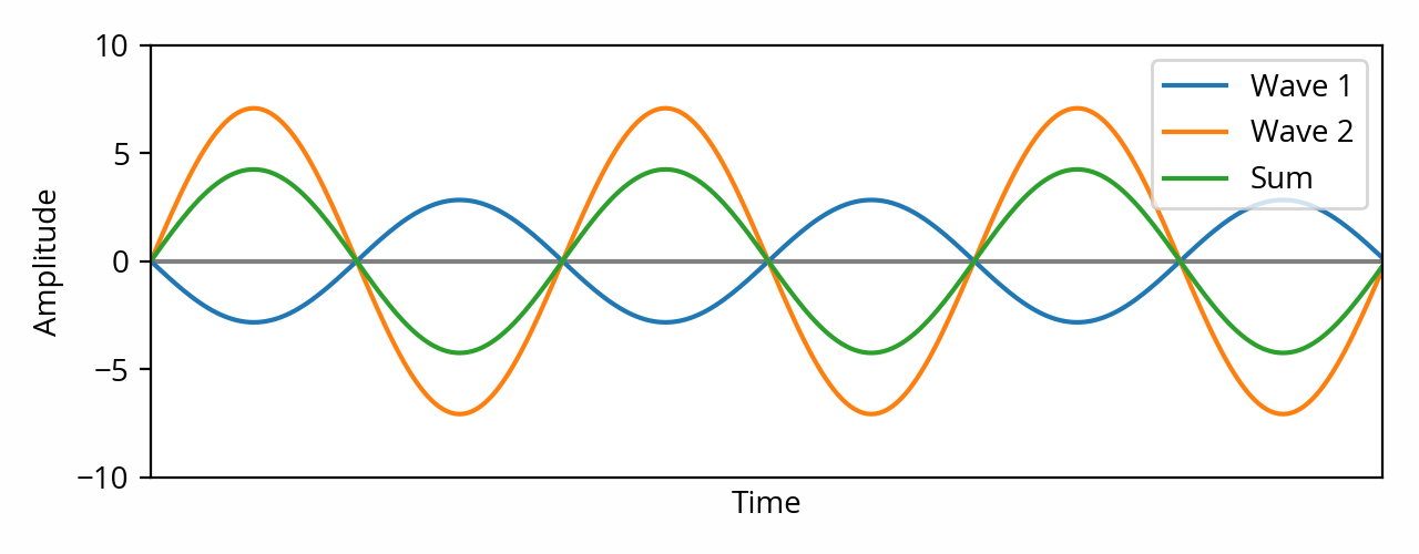
This time the peaks of one wave are aligned with the valleys of the other wave. This means their amplitudes subtract instead of add, which is why this is called destructive interference or cancellation. In the special case where the two waves have exactly the same amplitude, they cancel each other out perfectly, and the signal vanishes — the result is silence. Active noise control, the technology used in noise-canceling headphones, is an example of this phenomenon.
The sum of two sine waves that have identical frequency and opposite phase is itself a sine wave of that same frequency. The resulting amplitude (peak or RMS) is the difference between the two amplitudes. The resulting phase is the phase of the wave with the strongest amplitude.
Same frequency, arbitrary phase
When dealing with two sine waves of identical frequency, but neither identical nor opposite phase, we find ourselves deprived of a simple rule of thumb; there’s no avoiding the math in this case. However, the following plots will give you an idea as to what to expect. They describe the effect of summing two sine waves that differ by a particular amplitude ratio (line color) and phase (horizontal axis). The “same phase” case that we’ve seen in the first section is located in the middle of the horizontal axis, while its sides illustrate the “opposite phase” case that we’ve seen in the previous section.
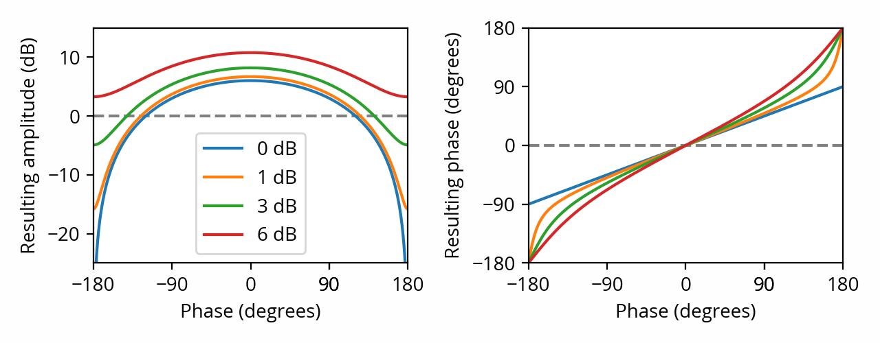
The sum of two sine waves that have identical frequency is itself a sine wave of that same frequency. The resulting amplitude and phase depend on the amplitude ratio and phase of the two waves.
Different frequencies
So far we’ve only been dealing with pure sine waves of identical frequency. What about the sum of sine waves of different frequencies?
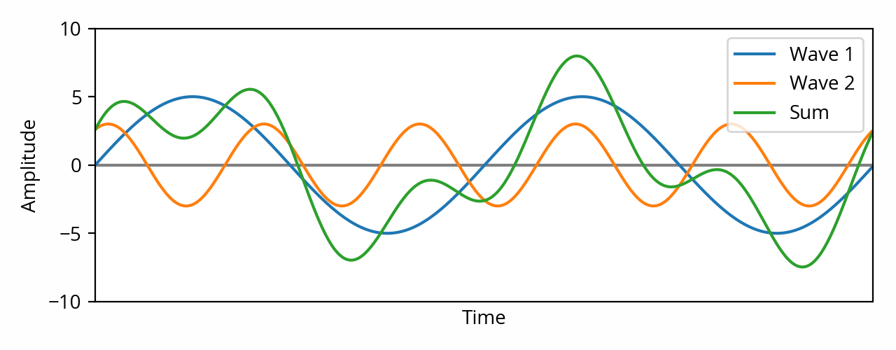
In this case, as illustrated by the above plot, the result is not a sine wave. We can see that the peak amplitude is the sum of the peak amplitudes of the two waves — here, 8 (5+3). This makes sense, because two sine waves of different frequency will, given enough time, eventually line up with each other such that their peaks are aligned, even briefly. [note] Here I’m assuming that the signal is of infinite duration, or at least sufficiently long that it makes little difference. If the signal is of limited duration, the peaks will not necessarily have the opportunity to line up, and the peak amplitude will therefore be lower. [end note]
RMS amplitude is less trivial. We can’t use the same trick as before because we’re not dealing with a single sine wave anymore — we’re dealing with a different wave shape. Mathematically there are many ways to derive the answer, but perhaps the most straightforward is to use the Parseval theorem, which basically states that the sum of squares of a waveform is equal to the sum of the squares of the sine waves (of different frequencies) that comprise it. In the above example, the RMS amplitudes of the original sine waves are approximately 3.5 and 2.1, so the RMS total is the square root of 12.5+4.5=17 — which is approximately 4.1.
The sum of two sine waves of different frequencies is not a sine wave. The peak amplitude of the resulting wave is the sum of the peak amplitudes of both sine waves. The RMS amplitude of the resulting wave is the RMS total of the amplitudes of both sine waves.
Arbitrary signals
Since any signal can always be decomposed into a sum of sine waves using the Fourier transform, the above section de facto provides a general solution that can be applied to any pair of signals: decompose both signals, add the sine waves at each frequency using the rules from the first three sections above, sum them back using the rule from the fourth section, and you’re done. [note] Granted, that’s not really easier than just adding the two waveforms directly, is it — especially since computing the Fourier transform without the help of a computer is, well, extremely hard. The point was to demonstrate the variety of approaches that can be used to think about these sums. Depending on the situation, some of these techniques may be easier to apply than others. [end note]
Caution: If you know the amplitude spectrum for the two signals that you want to sum, you might be tempted to simply add them together in the frequency domain, by summing the amplitude at each frequency. In most cases that’s incorrect, because at each frequency you are summing sine waves without knowing their respective phase — the actual result might be less than the sum of the amplitudes. The correct result can only be obtained by summing the raw complex output of the Fourier transform, which includes phase information, before extracting the amplitude information.
That said, there are cases where we can get away with a simpler approach. Consider a scenario in which the two signals are completely and utterly unrelated to each other; for example, it could be two noise signals, or two separates pieces of music, or the voice of a commentator on top of a soundtrack, or a notification sound playing on top of other content. The trick in that case is to see the two signals as two independent random processes, in the mathematical sense of the term. [note] The usual caveats apply, including the simplifying assumptions that the signals are truly unpredictable and extend infinitely in time. This is an approximation, albeit one that works well in practice. [end note]
From that perspective, peak amplitude is intuitively the sum of peak amplitudes, since, given enough time, two peaks will eventually align. As for RMS, the trick is to see that the sum of squares is just another name for the variance, of which RMS amplitude is the square root (which makes it the standard deviation). The variance of the sum of two independent random variables is the sum of the variances, so we can directly deduce that the RMS amplitude of the sum of two unrelated signals is the root of the sum of the squared RMS amplitudes — i.e. the RMS total. [note] The RMS total is also known as the power sum. This makes sense because power is proportional to the square of the amplitude. [end note] In that sense, summing two unrelated signals is similar to summing two sine waves of different frequencies as described in the previous section.
The peak amplitude of the sum of two unrelated signals is the sum of the peak amplitudes. The RMS amplitude of the sum is the RMS total of the amplitudes.
A word about decibels
At this point, I should warn you about decibels. Due to their logarithmic nature, decibels are great for manipulating ratios and multiplying things, but they tend to get in the way when doing additions. As a gentle reminder, the sum of, say, ×2 (6 dB) and ×5 (14 dB) is ×7, which is 17 dB, not 20 dB.
In fact, it gets even more confusing when you realize that what I just did in this example was directly summing two values, which is only a good idea in some of the cases that I’ve described above: namely, perfect constructive interference, or when dealing with peak amplitudes. It is not the correct approach when dealing with RMS totals. Which is really unfortunate, because decibel values are typically expressed in RMS, so the intuitive direct approach is wrong in many cases.
Fortunately, decibels can also help us in their own way, as they make it easier to express the amplitude of the sum when the ratio of the amplitudes of the original signals is known. For example, ×2 is +6 dB, which can help when summing signals of identical amplitude. What’s much more interesting, though, is that the RMS total of two signals of identical amplitude turns out to be their RMS amplitude multiplied by the square root of 2… which, conveniently, happens to be approximately +3 dB. If we combine that with the knowledge we gained in the earlier sections, we can say, for example, that summing two unrelated signals of equal amplitude results in a peak amplitude of +6 dB and an RMS amplitude of +3 dB above the original signals. Isn’t that nice?
In fact, we can summarize what we’ve just learned as follows:
| Sum of two signals of equal amplitude | Peak | RMS |
|---|---|---|
| Sine waves of identical frequency and phase | +6 dB | +6 dB |
| Sine waves of identical frequency and opposite phase | -∞ dB | -∞ dB |
| Sine waves of different frequencies | +6 dB | +3 dB |
| Unrelated signals | +6 dB | +3 dB |
These results can be extended to arbitrary ratios of amplitudes, and calculators exist to help you do just that, be it for the RMS total case or the direct (peak) case.
I’ll leave you with one last rule of thumb: decibels being a logarithmic unit, the contribution of a given term to the sum falls quickly as the decibels decrease. For example, the direct sum of 0 dB and -20 dB is only 0.8 dB. This can be used to dismiss the contribution of the smaller terms as negligible. [note] It’s also why low-level noise, which normally sits at -80 dB or less relative to the signal, has a negligible effect on the overall amplitude. [end note]