As the audio signal makes its way through the different realms of the system, it travels through various digital, analog, and acoustic components that alter the signal in various ways. Some of these alterations might or might not be audible, or might only be audible under certain conditions. In most scenarios relevant to this blog they are undesirable side effects from limitations in the components that make up the system, though in some specific cases they can be deliberately introduced in pursuit of a specific goal (e.g. equalization).
In order to build a high quality audio system, it is necessary to keep signal degradation (i.e. unwanted alteration) under control, and this requires a good understanding of what these alterations might be, what causes them, and how to avoid or alleviate them. Ever since the advent of sound reproduction more than a century ago this topic has been the subject of great debate, some thoughtful and innovative, some misguided or downright counter-productive. Hopefully this blog will do more of the former and less of the latter — but for now, this post serves as a brief introduction to the issues at hand.
Signal alterations can be divided into three broad categories: noise, frequency response distortion, and non-linear distortion. [note] When used by itself without qualification, the term “distortion” can refer to some or all of these categories, depending on context. [end note] Real-world systems exhibit all three kinds in varying amounts. What follows is a brief overview of the issues at hand; future posts will look at each of them more closely.
Noise
Noise describes an alteration of the signal in which a separate, unrelated signal is added (i.e. mixed in, superposed) to the original signal. [note] This is the definition I’ll use throughout this blog, pursuant to IEC 60268–2. In other contexts noise might be used in a more specific way (e.g. broadband noise only), or in a more general way (e.g. signal differences introduced by non-linear distortion are considered to be part of the noise signal). [end note] That additional signal has its own characteristics including amplitude and frequency content (spectrum), which are combined with the characteristics of the original signal. Noise is often quantified by comparing the amplitude of the noise to the amplitude of the signal, a metric known as the signal-to-noise ratio (the higher the better).
Noise can appear in all three of the audio realms. In the digital realm it can take the form of dithering noise for example, though modern digital systems provide good enough performance that noise sits comfortably below the threshold of audibility. This is not always the case in the analog realm, where noise problems are the most common, the most objectionable, and the most pernicious — often the result of complex electromagnetic interference phenomena, subtle hardware defects, or compatibility issues. Finally, the acoustic realm is rife with often overlooked sources of noise from ordinary life, from the rumbling of an air conditioning unit to the occasional car driving down the street.
Depending on amplitude and frequency content, noise might or might not constitute a problem in practice. For example, low-level broadband colored noise (such as white noise) will often go unnoticed because its spectrum is roughly similar to typical ambient noise that we are all continuously subjected to in our daily lives. [ref] See Albert Donald G., Decato Stephen N., “Acoustic and seismic ambient noise measurements in urban and rural areas”, Applied Acoustics, 119, 135–143, (2017) for examples of ambient noise spectra. [end ref] The same cannot be said of narrowband noise concentrated in specific frequencies. [note] Unfortunately that distinction is lost when noise measurements are condensed into a single number (such as signal-to-noise ratio), discarding spectral distribution in the process. [end note] Furthermore, narrowband noise is more likely to affect the perception of minute detail in the original signal, due to an auditory phenomenon known as masking.
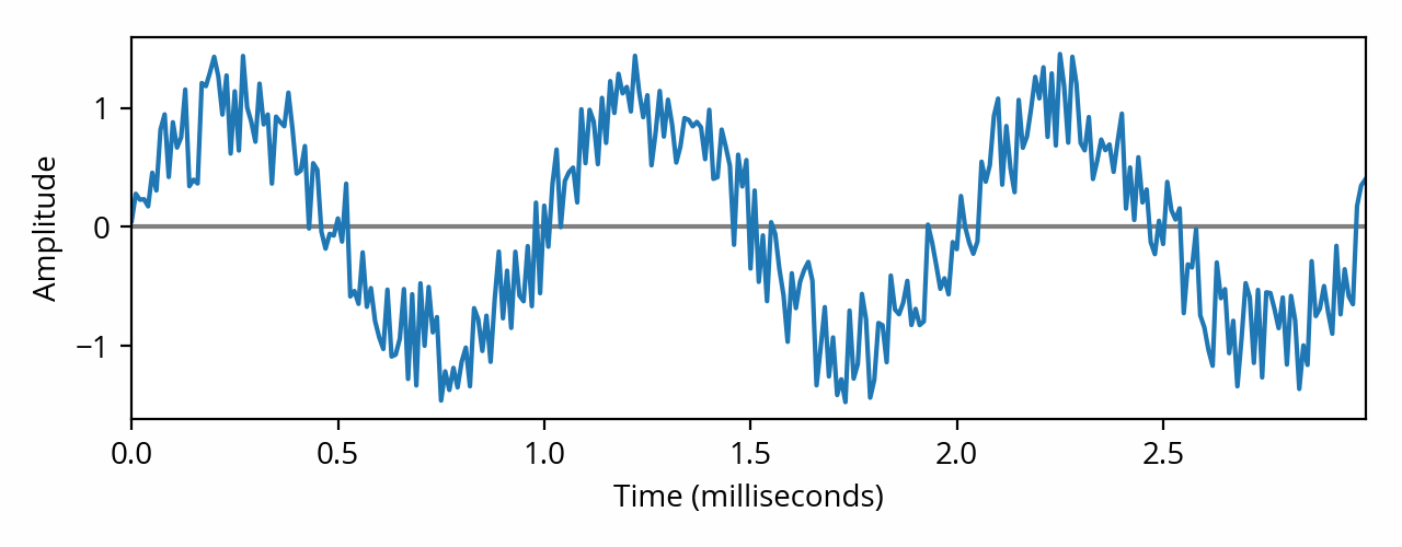
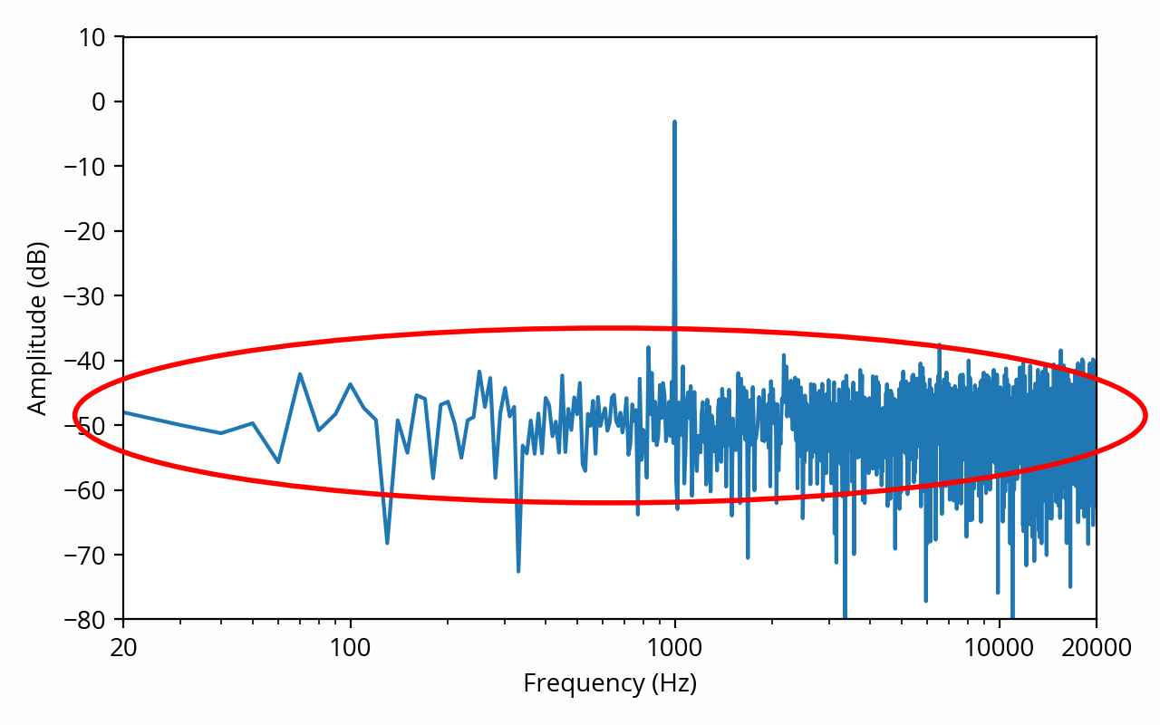
Waveform and spectrum of a sine wave affected by white noise. The noise spectrum, circled in red, is often called the “noise floor”. [note] From that spectrum plot you might be tempted to conclude that the signal-to-noise ratio is about 50 dB. That would be wrong — it’s actually much worse, around 17 dB. You can’t read it directly from the graph because the noise is spread across multiple frequencies. This is a very common mistake when reading spectrum plots, which I might describe in more detail in a future post. [end note]
In a real-world scenario, noise is only really noticeable when the original signal is relatively quiet, such as when there is a break in a piece of music, because all that remains is the noise itself. Conversely, noise is inaudible when a significantly loud signal is playing, again because of masking (but this time in reverse). In practice, I tend to abide by the following rule of thumb: if you can’t hear anything when playing a silent signal, then your system is probably fine as far as noise is concerned.
Frequency response distortion
In the first post on this site, I explained that an audio signal can be decomposed into a number of constituent signals of various frequencies. One way an audio component can alter the signal is by changing the amplitude (i.e. applying gain) on some of these frequencies more than others. This relationship between frequency and gain is known as the frequency response.
If this relationship is constant, i.e. the same amplitude multiplier is always applied to a given frequency regardless of the shape of the signal, then we are dealing with a linear time-invariant system. We can plot the frequency response on a graph, known as a frequency response graph (or, more technically, a Bode plot). [note] One thing that I’ve omitted to keep things simple is that a linear time-invariant system is not just allowed to change the amplitude of individual frequency components, it can also change their phase. This is conveyed through the phase response. Technically the term “frequency response” encompasses both magnitude response and phase response, though the latter is often dismissed for lack of relevance in most audio discussions. More on the phase response in the next post. [end note]
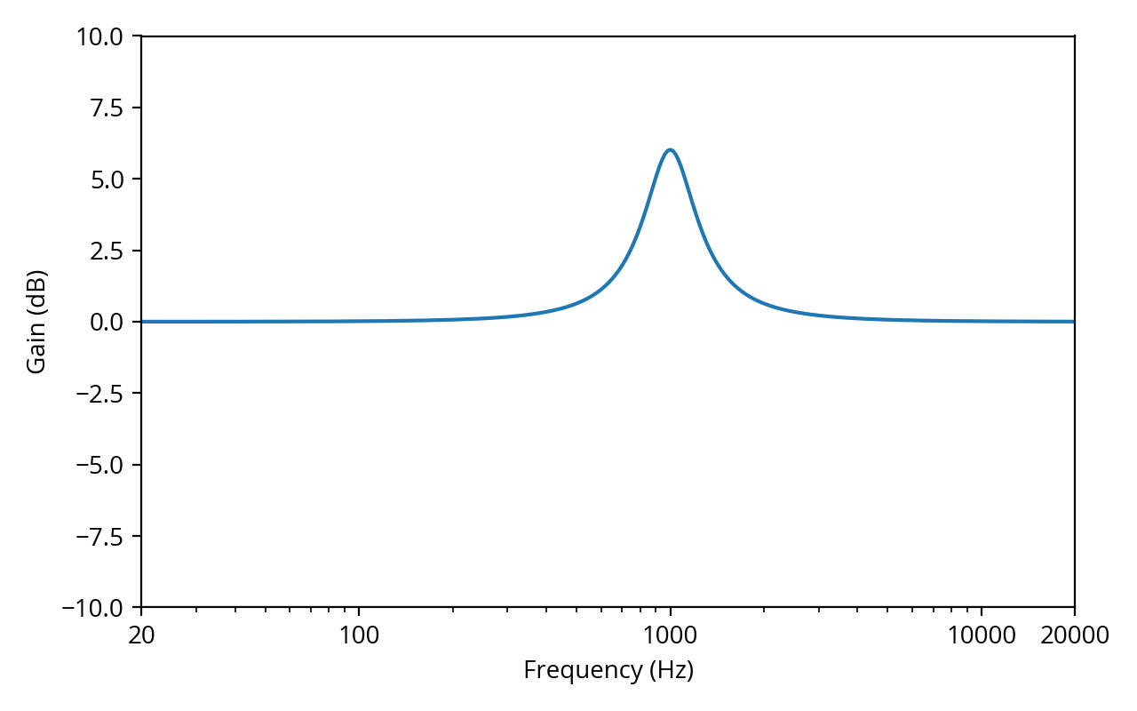
The frequency response of a system that amplifies frequencies around 1 kHz by about 6 dB. This particular type of distortion is called a resonance.
How is this useful? Well, remember that the frequency domain is often more useful than the time domain when it comes to understanding how audio signals are perceived. Frequency response tells us how a system alters the frequency components of the signal that flows through it. That makes it one the most powerful tools in the audio engineer’s toolbox.
Studies show that frequency response is extremely important when it comes to assessing audio quality in real-world scenarios. For example it has been shown that the human auditory system is capable of detecting frequency response variations as tiny as 0.1 dB [ref] Toole, F. and Olive. S., “The Modification of Timbre by Resonances: Perception and Measurement”, J. Audio Eng. Soc., 36(3), 122–141, (1988). From Fig. 9: coherent sum of 0 dB and -40 dB sources is ~0.1 dB. [end ref] , and that it is by far the most important criterion when it comes to assessing the quality of a loudspeaker [ref] Olive, Sean, “A Multiple Regression Model For Predicting Loudspeaker Preference Using Objective Measurements: Part 1 — Listening Test Results”, presented at the 116th AES Convention, Berlin, Germany, preprint 6113, (May 2004). [end ref] . Make no mistake: this metric is a huge deal, and I expect most posts on this blog will make use of it in one way or another.
The digital and analog realms typically contribute very little in the way of frequency response distortion. Virtually all of it is found in the acoustic realm, as even the best loudspeakers and headphones struggle to keep their frequency response within a few dB of the intended target [ref] Many examples can be found in the SoundStage database (loudspeakers) and the InnerFidelity database (headphones). [end ref] . It gets worse: the acoustics of home listening rooms (room modes especially) can result in low frequency alterations in the order of 10 dB or more! [ref] Literally any frequency response measurement made in a small room will show this phenomenon. One example can be found in Leduc Michel, 2009, “How Does Listening Room Acoustics Affect Sound Quality?“, Audioholics (graph under “Standing waves” section). A series of representative examples can be found in Toole, Floyd E., Sound Reproduction: Loudspeakers and Rooms, figure 13.9. [end ref] No wonder why these are often said to be the “weakest links” of the audio chain…
Non-linear distortion
Ideally, audio components should meet the definition of a linear system as described above; that is, they should be able to accurately track the input signal, such that the output is precisely proportional to the input. Of course that is not the case in practice. Besides noise (which we’ve already covered), consider, for example, that the driver inside a loudspeaker is made from imperfect materials that have imperfect physical properties, so its movement will not perfectly track the signal, instead giving rise to non-linear distortion. One example in the analog realm is crossover distortion that can occur in certain types of amplifiers.
Fortunately, any reasonable audio system will be at least approximately linear, so we can still use the frequency response to reason about the system. At the same time, we need to keep ourselves honest and account for any remaining non-linear behavior that might alter the signal in ways that frequency response and noise measurements will not predict. This is appropriately called non-linear distortion, also known as amplitude distortion.
This definition makes non-linear distortion a very open-ended category, as indeed a signal can be distorted in an infinite variety of ways. Since it is not possible to run an infinite number of tests, measuring and quantifying the non-linear behavior of a system can be quite challenging. That said, most non-linear distortion comes in well-known shapes and forms, so a few standard measurements are usually good enough to characterize the performance of an audio system.
One important aspect of non-linear distortion is that, contrary to frequency response distortion, it can cause new frequencies to appear that weren’t present in the original signal. By far the most well-known type of non-linear distortion is harmonic distortion, where new frequencies appear that are whole multiples (harmonics) of the frequencies in the original signal. It is often summarized in a single number, total harmonic distortion (THD), which indicates the total amplitude of the introduced harmonics relative to the original signal (more precisely, the fundamental). A related phenomenon is intermodulation distortion, where multiple frequency components in the signal interact with each other to create new frequencies in a specific pattern.
At the beginning of this section I described examples of non-linear distortion that can occur during normal system operation. However, the most egregious, obvious, and audible non-linear distortion issues occur when the system is driven beyond its limits; that is, signal amplitude is pushed too far and the system is unable to keep up. When this happens the peaks of the waveform cannot be reproduced faithfully and the system “bottoms out”, a phenomenon known as clipping. To mention a few examples, this can happen in the digital realm (which is otherwise immune from most other forms of non-linear distortion) due to overflowing the largest possible sample value; in the analog realm due to exceeding the power limits of an amplifier; or in the acoustic realm due to exceeding the movement limits of a driver (excursion).
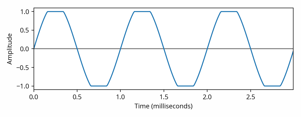
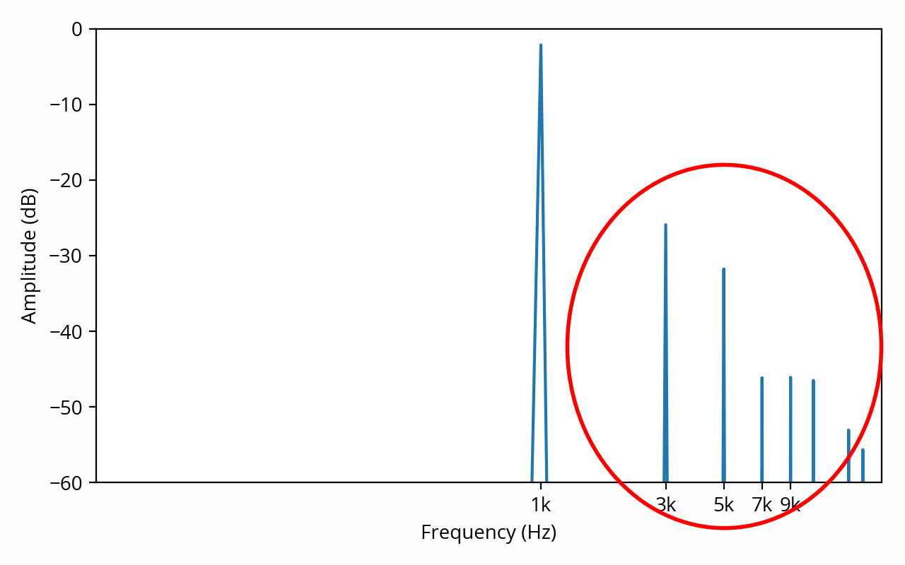
Waveform and spectrum of a 1 kHz sine wave showing symptoms of “hard clipping”, which produces odd-order harmonics (circled in red). The THD in this example is about 7%. [note] Here’s how this number is calculated. First, take the RMS amplitude of the harmonics: 3 kHz -26 dB (0.051) 5 kHz -32 dB (0.025) 7 kHz -46 dB (0.0047) 9kHz -47 dB (0.0043)… the total RMS amplitude of the harmonics is 0.057. The RMS amplitude of the fundamental is 0.78. The THD is the ratio of these two numbers, which is 0.073, or 7.3%. [end note]
So how audible is non-linear distortion? Well, that depends. Because non-linear distortion can take many forms, there is no simple answer. For example, distortion in the lower frequencies is less audible than in higher frequencies, and it is less audible if the newly introduced frequencies are close to the fundamental (thanks, once again, to masking). [ref] Temme, Steve, “Application Note: Audio Distortion Measurements“, Brüel & Kjær, 1992. [end ref] Condensing non-linear distortion measurements into a single, simplistic THD number, as is often done, certainly doesn’t help. With that in mind, real-world examples tend to suggest that a THD of 10% is likely to be audible, 1% is borderline, and 0.1% is unlikely to be audible. [ref] Audioholics, ”Human Hearing - Distortion Audibility Part 3”, 2005. [end ref]