In previous posts about the acoustic realm, we’ve assumed that sound propagates into free space, willfully ignoring the pesky issue of obstacles or walls getting in the way. Such simplifying assumptions will only get us so far, if only for the fact that the inside of your living room is not levitating in free space. We need to take a close look at what happens when sound comes into contact with something other than air. But before we go there, we need to examine exactly how sound propagates in air — or any other fluid for that matter; that is the focus of this post. From there it will be easier to explain what happens when obstacles enter the picture.
Plane waves
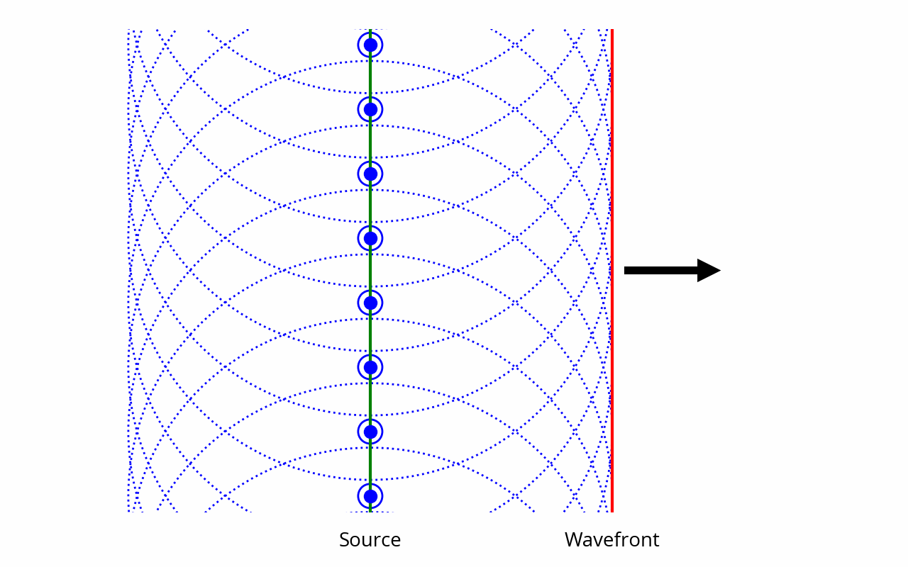
In previous posts, we’ve been assuming sound is being produced by a point source. Conceptually, point sources are like infinitely small balloons (spheres) that contract and expand to produce a sound wave around them, thus producing a spherical wavefront.
While these concepts served us well, there are cases, such as in this post, where the technicalities of dealing with spheres can get in the way of understanding. For this reason, in this post we’re going to visualize a wavefront as a flat plane (or a line in 2D). This is called a plane wave. To create such a wavefront, one could use a vibrating membrane, just like in a typical loudspeaker driver, in lieu of a pulsating balloon.
At first glance this approach might seem disconnected from the spherical waves we’ve been using before. This is not so: there are ways to bridge these two. Specifically, a plane source can be represented as an infinite set of point sources: [note] The general idea of using a set of point sources to approximate a complex wavefront goes much farther than this, as evidenced by the Huygens-Fresnel principle. [end note]
Furthermore, a sufficiently small portion of a spherical wavefront can be approximated as a planar wavefront:
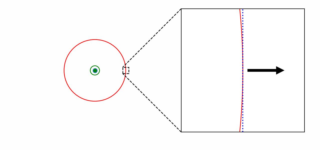
Part of what makes plane waves simpler is that they are not subject to the inverse square law, because, contrary to an expanding sphere, sound power doesn’t get spread over a larger surface as the wave progresses. This is consistent with the above diagram: when looking at a spherical wavefront on a scale that is much smaller than the radius, then, by definition, the distance to the source doesn’t change much, and as a result the inverse square law can be neglected. This progressively ceases to be true as we zoom out. In the reminder of this post we are also going to ignore the small effect of air attenuation to avoid distractions.
When dealing with plane waves, it is often assumed, for simplicity’s sake, that the wavefront has infinite extent, i.e. it’s a literal geometrical plane. Said differently, it is assumed that the planes — and, by extension, the sound source that’s producing them — extend much farther than the phenomenon we’re studying, such that it doesn’t matter what’s happening at the edges. As usual, this simplifying assumption does not fundamentally affect the phenomena that we’ll be studying in this post; it just makes things more focused and easier to visualize.
Modeling air
Our goal in this post is to understand what’s going in a volume of air as sound travels through it.
“What’s going on in a volume of air” is one of the most vague and all-encompassing questions one could possibly ask. Let’s say we want to study the propagation of a simple 1000 Hz sine wave, which has a wavelength of ~340 millimeters. A cubic millimeter of air contains about 10¹⁶ (ten million billion) molecules. Since air is a gas, these molecules are constantly moving around in mostly random fashion. Clearly, trying to understand what’s going on by looking at individual molecules — on a microscopic scale — sounds like a tall order.
Instead, it makes more sense to look at the behavior of air on a macroscopic scale. For the distances we are dealing with, the number of molecules is large enough that the overall behavior emerging from their random interactions can be statistically summarized through a few simple metrics, such as density, temperature and pressure. Among these metrics, the one we care about the most is of course pressure — remember that pressure variation is the very definition of sound itself.
That said, for the purposes of our investigation, it wouldn’t make sense to go to the other extreme and study the entire volume of air as a single unit. Indeed, sound waves are pressure fluctuations that propagate through space; if we only look at the overall pressure of the entire volume of air, information about these local fluctuations is lost.
Therefore, it looks like the best way to approach this problem is to strike a compromise. We will arbitrarily divide the space into a number of individual “pockets” of air of constant mass, each with its own properties. The idea is to study a complex system by breaking it down into simple constituent parts and examining their interactions. [note] This general approach is not just useful for educational purposes, mind you. It forms the basis of how physical laws are applied by engineers and scientists to study the behavior of complex systems, using techniques like the finite element method or the finite difference method. The acoustics of loudspeakers and concert halls, for instance, are often designed using such methods. [end note] These pockets of air should be small enough that we can clearly see the propagation of the sound wave through space, but not too small lest we lose sight of the big picture. Here, for our 1000 Hz wave, it would be enough to have pockets that are, say, around 17 mm in size, such that a single wavelength is broken down into 20 pockets or so.
Initial setup
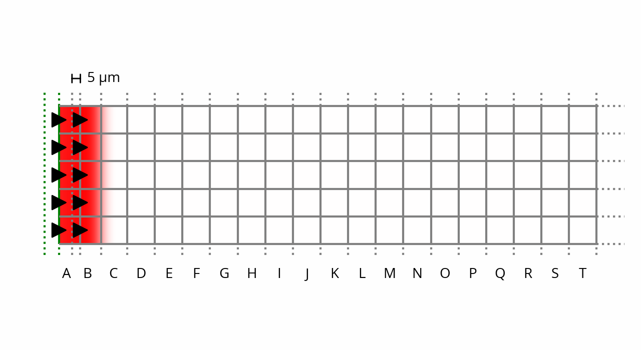
Let’s set the stage as a single vertical plane wave source, i.e. an infinitely large membrane, situated on the left and vibrating laterally in a free field. The goal is to study what’s happening to the air pockets situated on the right of that membrane. Here is a 2D projection along with a grid of cubic air pockets:
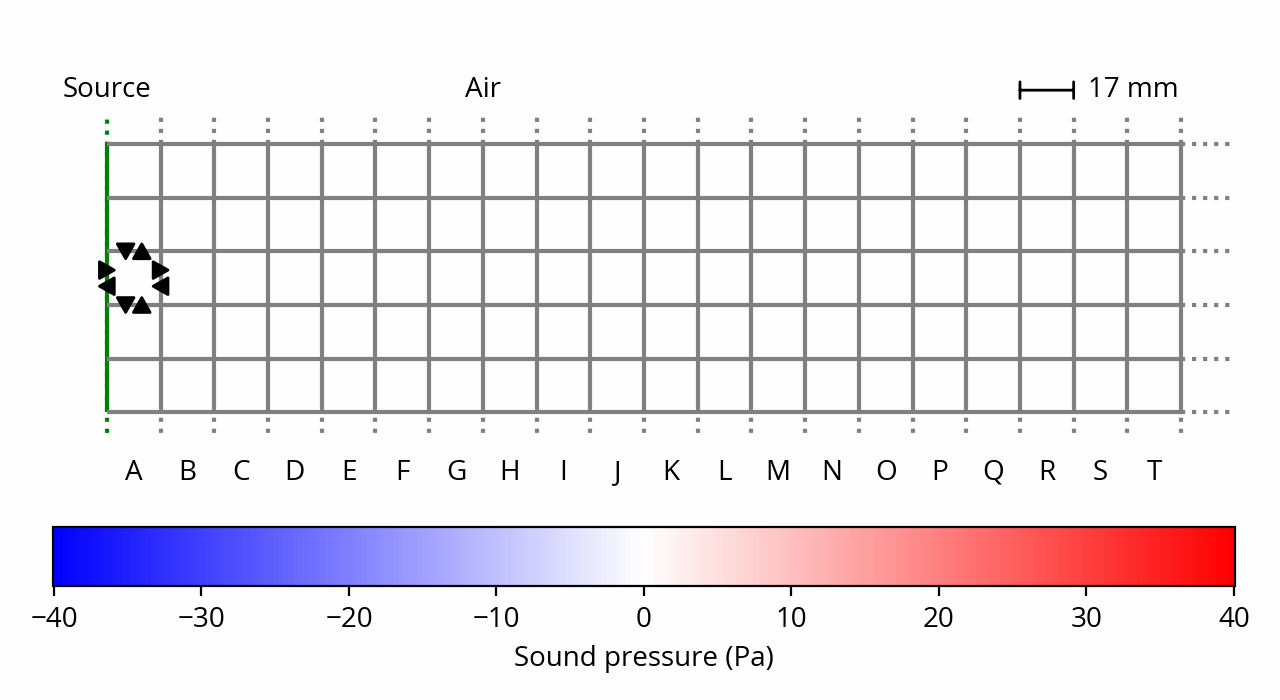
Air is under ambient (atmospheric) pressure, which in practice means that our little air pockets want to expand outwards; in other words, each air pocket exerts a force on its neighbors — that force is the very definition of what pressure is. It is represented by black arrows on the above plot, for one example air pocket.
However, since all our air packets apply the same force on each other, everything cancels out, and nothing happens — the gas is at rest. This is still true in the presence of the membrane, if we assume that it is locked into position. [note] If we assume that there is air on the left on the membrane, then there would be pressure on the membrane from the left side too, and it would have no reason to move anyway. This is not pictured above as I want to focus on what’s happening on the right side of the membrane. [end note] In this initial state, pressure is the same everywhere, therefore the sound (relative) pressure is zero everywhere, and everything is silent. In the remaining of this post I will mostly ignore ambient pressure to focus on sound pressure.
What happens if we start moving the membrane?
Compression
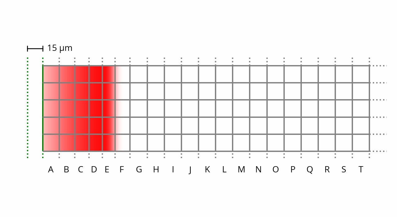
As already decided, we’re going to make our membrane vibrate at a frequency of 1 kHz. We also need to decide on an amplitude of vibration, let’s say 15 micrometers (peak). This is called the displacement of the membrane. [note] This might seem very small, but as we’ll see below, even a minuscule displacement can sound quite loud. This is the reason why a loudspeaker membrane doesn’t seem to be vibrating to the naked eye. Except perhaps low-frequency subwoofers, which, for equal sound pressure, require higher displacement because the wavelength is longer. [end note] For the purposes of this post, we’re going to assume that the motion of the membrane is irresistible, i.e. it will move at its own pace whether the surrounding air likes it or not. [note] I’m not going to discuss this assumption here, because the behavior of sound sources is a story for a different post. I’ll just mention in passing that this is consistent with how a typical loudspeaker driver would behave. [end note]
Like a bulldozer, the membrane will displace any air particle that stands in its way. These particles will accumulate in front of the membrane; as a result, the air pockets in front of the membrane (column A) become denser. But remember that we’ve defined our air pockets as having constant mass; if they become denser, that necessarily means that their volume will decrease. In other words, we have compression. Behold, as we are now entering the world of thermodynamics.
This is how things look like when the sine wave is at 5% of its cycle. About 50 microseconds have elapsed, and the membrane has moved by about 5 micrometers. [note] Yes, the membrane has traveled a third of the way in 5% of the time. That’s because a sine wave starts fast, but slows down as it approaches its peak. [end note] Notice the compression of column A:
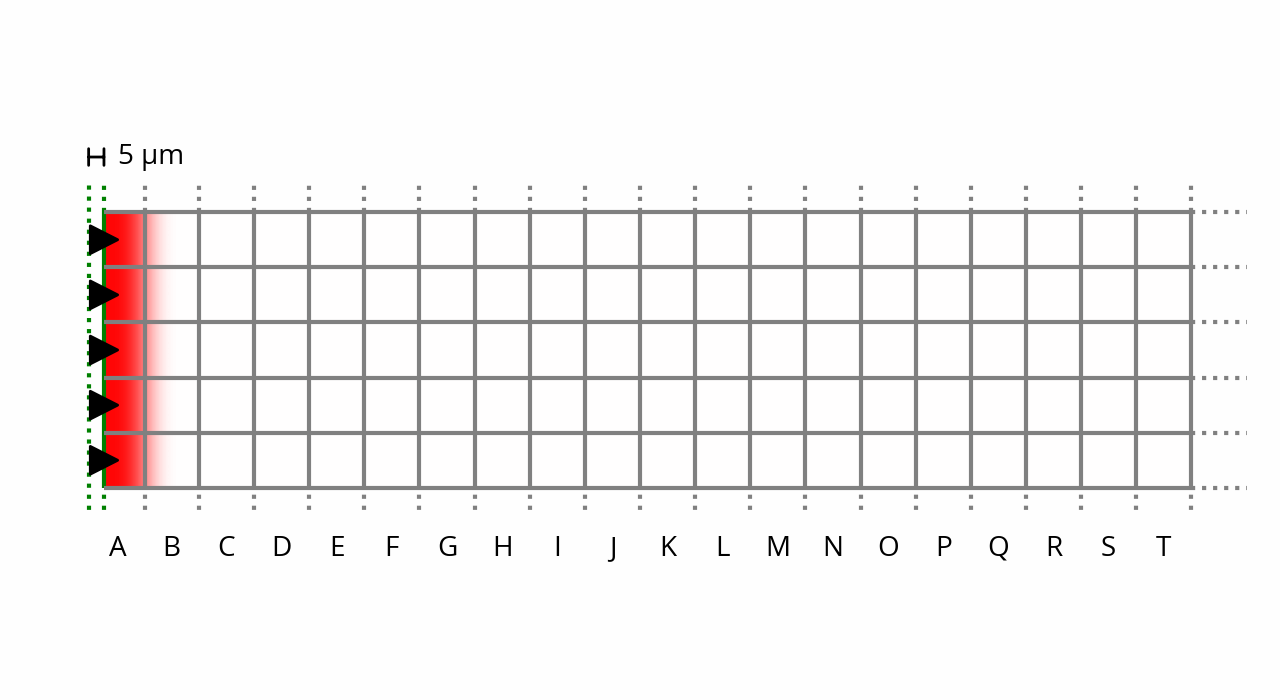
Note that, in order to make the compression visible, these plots are not to scale: the displacement amplitude is magnified by a factor of 1,000 compared to reality.
Remember that a gas is just a collection of fast-moving particles that are constantly colliding with one another and with its boundaries. If one of our constant-mass gas pockets shrinks in volume, then the particles it contains, being confined into a smaller space, will collide with each other and with the surroundings more often and with more energy. This means that the temperature and pressure of the air pocket will increase.
These changes in volume come and go at such a rapid pace that the air pockets don’t have any time to exchange heat to each other; this means we are dealing with an adiabatic process. [ref] Beranek, Leo L., Acoustic measurements, §2.2.J (page 49). Beranek, Leo L., Acoustics: Sound Fields and Transducers, §2.2.2 (page 24). Also see “Why are sound waves adiabatic?” for a more detailed treatment of the question. [end ref] This makes things easier, because it means the pressure can be deduced directly from the volume. Indeed, in such a process, pressure is inversely proportional to volume to the power of the adiabatic index, which in the case of air is about 1.4.
So let’s apply this reasoning to the situation shown on the plot above. Remember that our pockets are normally ~16 mm in length, but the ones in column A have been compressed by ~5 µm lengthwise, a ~0.03% reduction in volume. This is such a tiny change that the exponent can be approximated as a linear factor, leaving us with pressure inversely proportional to volume. In fact, this approximation is precisely what allows us to assume air is linear so long as sound pressure is not increased to eardrum-splitting levels. [ref] Beranek, Leo L., Acoustic measurements, §2.8 (page 80). Thuras, “Extraneous Frequencies Generated in Air Carrying Intense Sound Waves”, The Journal of the Acoustical Society of America 1935 6:3, 173–180. [end ref]
And with that, finally, we can quantify the average sound pressure in column A at this instant: it’s about 0.04% of ambient pressure, or ~40 Pa (~125 dB SPL). This value show up as red on the plot.
So far so good. What happens next?
Propagation
Let’s go back once again to the definition of pressure: it’s the force that air pockets exert on their neighbors. We’ve just concluded that pressure inside the air pockets in column A has increased, which means they are pushing outwards with more force compared to the air at ambient pressure.
This additional force has no effect on the membrane, since we’ve decided that its motion is irresistible. It doesn’t have any effect along column A either, because all the air pockets in this column are in the same boat, so the forces they exert on each other cancel out.
The same cannot be said of column B, however. That column is feeling less force from column C on the right, which is still at ambient pressure, than from pressurized column A on the left. This force doesn’t cancel out and is acting to push column B towards the right. According to Newton’s second law, this will result in the air in B accelerating to the right — the amount of acceleration is the total force divided by the mass (density) of air.
One interesting observation we can make at this point is that air particles in B are not being displaced in lockstep with the particles in A: the compression in A determines the acceleration of compression in B, not the compression itself. This hints at a time delay between events in A and events in B, which in the end just means the speed of sound is finite.
Since we know the force (pressure) from A, and we know the mass of an air pocket, we could be tempted to use Newton’s formula to determine the average acceleration of air particles in column B. From there, we should be able to determine particle velocity, and thus displacement, in B, after a certain amount of time has passed. We could then deduce the change in volume, and from there the change in pressure using the same reasoning as above, thus completing the cycle.
Now, it would be great if it was that simple, but it’s not. The problem is that while that “certain amount of time” passes, the parameters of our problem are continuously evolving, throwing our neat calculation into disarray. The membrane is not standing still during this time and keeps moving to the right, increasing pressure in A further, which changes the force that A exerts on B. Furthermore, we need to keep in mind what happens in B while it’s being compressed: we’ve determined earlier that a decrease in volume results in a proportional increase in pressure. The additional pressure in B pushes back against A, reducing the total force that B is subjected to. [note] In that sense the air in B behaves like a spring: indeed, pushback force (here, additional pressure in B) is proportional to distance from equilibrium (here, change in volume), which means we can directly apply Hooke’s law. This is why sound propagation is often explained by using the analogy of weights interconnected by springs. [end note] So, to recap, we have:
- The mounting pressure in A, which exerts an increasing force on B, compelling it to accelerate;
- The mass (density) of air in B, which constitutes inertia, reducing the acceleration;
- The mounting pressure in B, pushing back against the force from A, gradually reducing the acceleration as B gets compressed.
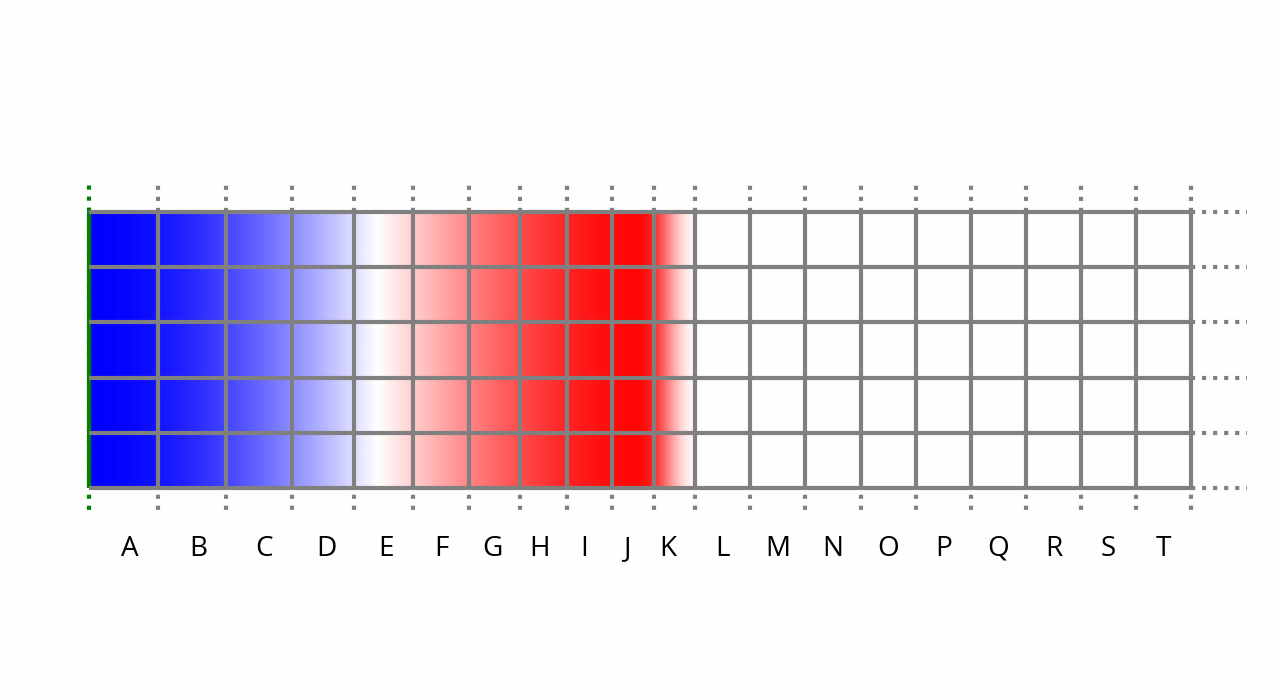
Numerically, the only direct way to figure out what happens at this point is to advance our “simulation” by very small time increments, recalculating the various forces, velocities and displacements at every step of the way. This would of course be quite tedious, which is why mathematical tools were invented precisely to solve this kind of problem: calculus, and in particular differential equations. If we combine Newton’s second law with the law governing adiabatic processes, we end up with the acoustic wave equation. Solving that equation at t = 50 µs results in the above plot, and if we advance time by a further 50 µs, we get the following:
The acoustic wave equation is the very essence of the phenomenon of sound propagation. It provides the fundamental basis for many properties of sound waves, including the fact that perturbations are allowed to travel through space undisturbed — this is illustrated by the 5 µm displacement of the membrane from 50 µs ago simply moving to the right with no other changes. [note] Of course, in the real world there would be attenuation, as we’ve seen in a previous post, but that’s still a linear change that doesn’t affect the shape of the wave. [end note] The sum of two solutions that satisfy the equation — i.e. two waves — is itself a wave: that’s the foundation for the superposition principle and acoustical interference phenomena.
The equation also provides a way to quantify the speed of propagation. Remember that the adiabatic index — or, more generally, the bulk modulus, or compressibility — determines how much pressure (force) results from a given change in volume, and that force increases acceleration of air particles; meanwhile, their mass creates inertia, which decreases it. Therefore, it should come as no surprise that the formula for the speed of sound, deduced from the wave equation, is a simple combination of these two parameters.
Towards steady state
Let’s fast forward to peak displacement of the membrane, at 25% of the cycle, t = 250 µs:
One thing to note here is that sound pressure in front of the membrane has decreased to zero. This is because the membrane is barely moving at this point, as it has reached the crest and is about to rush back towards its initial position. As a result, the air in front of the membrane had time to expand back to ambient pressure. This leads to the observation that when displacement is at peak, pressure is near zero, and vice-versa. An equivalent way to state this, since we’re dealing with a sine wave, is that displacement lags 90° behind pressure.
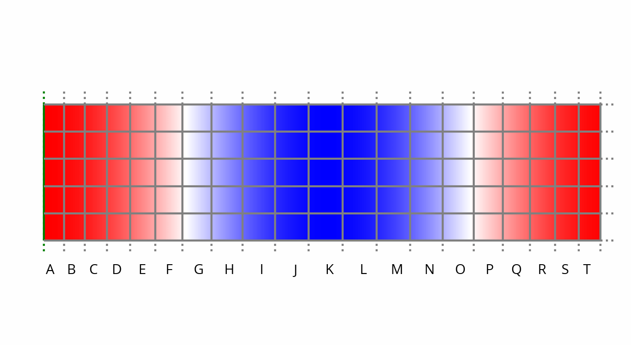
Let’s fast forward further, to 50% of the cycle, t = 500 µs:
The membrane went back to its original position. By doing so, it briefly leaves a vacuum in its wake, leading to an imbalance of forces, since the membrane is not pushing back against air pressure anymore. As a result, the air to the right of the membrane expands further to fill the gap: we have rarefaction, the opposite of compression.
And finally, after a full cycle, t = 1,000 µs:
And we’re back to where we’re started. At this point in time, if the membrane stops moving, the leftmost columns will again expand, restoring normal ambient pressure and pushing the high pressure region to the right. If the membrane continues pushing right instead, a new sine wave cycle begins anew.